Measuring Well-being

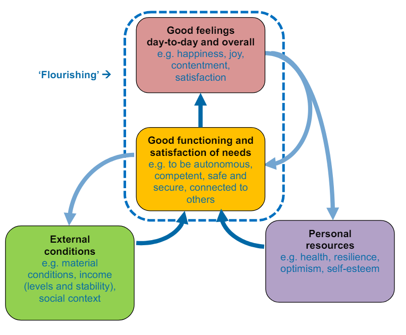
Well-being can be understood as how people feel and how they function, both on a personal and a social level, and how they evaluate their lives as a whole.

An individual’s external conditions – such as their income, employment status and social networks – act together with their personal resources such as their health, resilience and optimism – to allow them to function well in their interactions with the world and therefore experience positive emotions. When people function well and experience positive emotions day-to-day and overall, we can think of them as ‘flourishing’.

nef's dynamic model of well-being

1. GDP and its components as a measure of material well-being

GDP measures the monetary value of final goods and services—that is, those that are bought by the final user—produced in a country in a given period of time. It counts all of the output generated within the borders of a country.

Investigating GDP as well-being measure

We will examine GDP data from the UN’s National Accounts Main Aggregates Database, covering all countries from 1970 to now. We’ll analyze changes in GDP and its components over time and assess the usefulness of GDP per capita as a well-being measure.

UN = read_excel("gdp-usd-countries.xlsx",
  sheet = "Download-GDPconstant-USD-countr", 
  skip = 2)

Code Explanation:

This code imports the dataset into the project for further analysis.

The data-set looks something like this:

## # A tibble: 6 × 56
##   CountryID Country     IndicatorName  `1970` `1971` `1972` `1973` `1974` `1975`
##       <dbl> <chr>       <chr>           <dbl>  <dbl>  <dbl>  <dbl>  <dbl>  <dbl>
## 1         4 Afghanistan Final consump… 3.08e9 2.96e9 2.88e9 3.19e9 3.41e9 3.51e9
## 2         4 Afghanistan Household con… 2.71e9 2.60e9 2.52e9 2.79e9 3.00e9 3.03e9
## 3         4 Afghanistan General gover… 3.31e8 3.39e8 3.57e8 3.74e8 3.83e8 5.31e8
## 4         4 Afghanistan Gross capital… 1.69e9 1.81e9 1.58e9 1.58e9 2.03e9 2.35e9
## 5         4 Afghanistan Gross fixed c… 1.69e9 1.81e9 1.58e9 1.58e9 2.03e9 2.35e9
## 6         4 Afghanistan Exports of go… 1.80e8 2.32e8 2.77e8 3.48e8 4.79e8 5.05e8
## # ℹ 47 more variables: `1976` <dbl>, `1977` <dbl>, `1978` <dbl>, `1979` <dbl>,
## #   `1980` <dbl>, `1981` <dbl>, `1982` <dbl>, `1983` <dbl>, `1984` <dbl>,
## #   `1985` <dbl>, `1986` <dbl>, `1987` <dbl>, `1988` <dbl>, `1989` <dbl>,
## #   `1990` <dbl>, `1991` <dbl>, `1992` <dbl>, `1993` <dbl>, `1994` <dbl>,
## #   `1995` <dbl>, `1996` <dbl>, `1997` <dbl>, `1998` <dbl>, `1999` <dbl>,
## #   `2000` <dbl>, `2001` <dbl>, `2002` <dbl>, `2003` <dbl>, `2004` <dbl>,
## #   `2005` <dbl>, `2006` <dbl>, `2007` <dbl>, `2008` <dbl>, `2009` <dbl>, …

1.1 Assessment of Data

The data-set under examination encounters significant challenges due to missing data, which can be attributed mainly to political transitions and issues related to data availability. Notably, certain countries, especially those that emerged post-1970, demonstrate discontinuities within their data series.

We take the following steps to resolve this issue:

wide_UN <- UN
wide_UN = wide_UN[, -1]


long_UN = 
  melt(wide_UN, id.vars = c("Country", "IndicatorName"),
  value.vars = 4:ncol(UN))
names(long_UN)[names(long_UN) == "variable"] <- "Year"

Code Explanation:

Initially, this code snippet duplicates the dataset named UN into a new dataset called wide_UN and subsequently eliminates its first column. Following this, it transforms wide_UN from a wide format to a long format by utilizing the melt function. During this process, it retains "Country" and "IndicatorName" as identifier variables and consolidates the columns from the 4th to the last into a singular "Year" column. Ultimately, it renames the column that denotes the years from "variable" to "Year" to enhance clarity.

What was the need to reshape the data-set?

For many data operations and making charts it is more convenient to have indicators as column variables, so we would like Final Consumption Expenditure to be a column variable, and year to be the row variable.

To change data from wide to long format, we use the melt command from the package reshape2

The reshaped long data-set looks something like this:

##       Country
## 1 Afghanistan
## 2 Afghanistan
## 3 Afghanistan
## 4 Afghanistan
## 5 Afghanistan
## 6 Afghanistan
##                                                                              IndicatorName
## 1                                                            Final consumption expenditure
## 2 Household consumption expenditure (including Non-profit institutions serving households)
## 3                                         General government final consumption expenditure
## 4                                                                  Gross capital formation
## 5       Gross fixed capital formation (including Acquisitions less disposals of valuables)
## 6                                                            Exports of goods and services
##   Year      value
## 1 1970 3083688954
## 2 1970 2714637042
## 3 1970  330701239
## 4 1970 1693835531
## 5 1970 1693835531
## 6 1970  179671683

Creating Frequency Table showing the number of years that data is available for each country in the category ‘Final consumption expenditure’

cons = subset(long_UN,
  IndicatorName == "Final consumption expenditure")

Code Explanation:

This code calculates the number of available years of data for "Final consumption expenditure" indicator by country:

Subset Data: It selects rows from long_UN where IndicatorName is “Final consumption expenditure” and stores the result in cons.

Calculate Availability: It groups cons by Country, counts the non-missing (!is.na(value)) values in the value column (which presumably holds the expenditure data), sums them up for each country, and stores the result in available_years.

Finally, it prints the summarized data showing the number of available years of data for each country.

missing_by_country = cons %>%
  group_by(Country) %>%
  summarize(available_years=sum(!is.na(value))) %>%
  print()

## # A tibble: 220 × 2
##    Country             available_years
##    <chr>                         <int>
##  1 Afghanistan                      53
##  2 Albania                          53
##  3 Algeria                          53
##  4 Andorra                          53
##  5 Angola                           53
##  6 Anguilla                         53
##  7 Antigua and Barbuda              53
##  8 Argentina                        53
##  9 Armenia                          33
## 10 Aruba                            53
## # ℹ 210 more rows

Now we can establish how many of the 220 countries in the dataset have complete information. A dataset is complete if it has the maximum number of available observations (max(missing_by_country$available_years)).

result <- sum(missing_by_country$available_years == max(missing_by_country$available_years))
print(result)

## [1] 179

Hence there are 179 countries in the dataset that have complete information.

1.2 Calculation of GDP

There are three different ways in which countries calculate GDP for their national accounts, but we will focus on the expenditure approach, which calculates gross domestic product (GDP) as:

GDP = (Household Consumption Expenditure) + (General government final consumption expenditure) + ( Gross Capital Formation) + (Exports - Imports)

Household Consumption Expenditure:

Household consumption expenditure covers all purchases made by resident households (home or abroad) to meet their everyday needs: food, clothing, housing services (rents), energy, transport, durable goods (notably cars), spending on health, on leisure and on miscellaneous services.

General Government final Consumption Expenditure:

Government final consumption expenditure (GFCE) is an aggregate transaction amount on a country’s national income accounts representing government expenditure on goods and services that are used for the direct satisfaction of individual needs (individual consumption) or collective needs of members of the community (collective consumption).

Gross Capital Formation

Gross capital formation refers to the creation of fixed assets in the economy (such as the construction of buildings, roads, and new machinery) and changes in inventories (stocks of goods held by firms).

Calculating Net exports

Typically, instead of examining exports and imports independently, we consider the difference between them, which is referred to as net exports.

long_UN$IndicatorName[long_UN$IndicatorName == 
  strwrap("Household consumption expenditure (including 
    Non-profit institutions serving households)")] <- 
  "HH.Expenditure"

long_UN$IndicatorName[long_UN$IndicatorName == 
  "General government final consumption expenditure"] <- 
  "Gov.Expenditure"

long_UN$IndicatorName[long_UN$IndicatorName == 
  "Final consumption expenditure"] <-
  "Final.Expenditure"

long_UN$IndicatorName[long_UN$IndicatorName == 
  "Gross capital formation"] <-
  "Capital"

long_UN$IndicatorName[long_UN$IndicatorName == 
  "Imports of goods and services"] <-
  "Imports"

long_UN$IndicatorName[long_UN$IndicatorName == 
  "Exports of goods and services"] <-
  "Exports"

table_UN <- dcast(long_UN, Country + Year ~ IndicatorName)
table_UN$Net.Exports <- 
  table_UN[, "Exports"]-table_UN[, "Imports"]

Code Explanation:

Renaming of Indicators:

The variable long_UN$IndicatorName undergoes renaming to more succinct names, tailored to specific economic indicators through conditional replacements.

Data Reshaping (dcast):

The dataset long_UN is reshaped into table_UN using the dcast function, transforming it from a long format to a wide format, where rows represent countries and years, and columns represent economic indicators.

Net Exports Calculation:

A new column, Net.Exports, is created in table_UN by calculating the difference between Exports and Imports.

Charts to show the GDP components

We examine the dynamics of GDP components for different countries using various visual figures like charts to get a better understanding of how different components affect the GDP and vice versa.

comp = subset(long_UN, 
  Country %in% c("United States", "China"))

comp$value = comp$value / 1e9

comp = subset(comp, 
  select = c("Country", "Year",
    "IndicatorName", "value"),
  subset = IndicatorName %in% c("Gov.Expenditure", 
  "HH.Expenditure", "Capital", "Imports", "Exports"))

library(ggplot2)


pl = ggplot(subset(comp, Country == "United States"),
  aes(x = Year, y = value))

pl = pl + geom_line(aes(group = IndicatorName, 
  color = IndicatorName), size = 1)

pl = pl + scale_x_discrete(breaks=seq(1970, 2016, by = 10))
pl = pl + scale_y_continuous(name="Billion US$")
pl = pl + ggtitle("GDP components over time")

pl = pl + scale_colour_discrete(name = "Components of GDP",
  labels = c("Gross capital formation", "Exports",
    "Government expenditure", "Household expenditure",
    "Imports")) 

pl = pl + theme_bw()

pl = pl + annotate("text", x = 37, y = 850,
  label = "Great Recession")

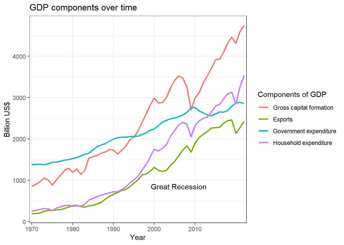
pl

US’s GDP components

Observation: From the above graph, we observe one very interesting thing about how various components affect GDP.

During the period of the Great Recession, significant components such as household expenditure, gross capital formation, and exports declined. However, to mitigate the effects of the recession, government expenditure was increased.

comp = subset(long_UN, 
  Country %in% c("United States", "China"))

comp$value = comp$value / 1e9

comp = subset(comp, 
  select = c("Country", "Year",
    "IndicatorName", "value"),
  subset = IndicatorName %in% c("Gov.Expenditure", 
  "HH.Expenditure", "Capital", "Imports", "Exports"))

library(ggplot2)


pl = ggplot(subset(comp, Country == "United States"),
  aes(x = Year, y = value))

pl = pl + geom_line(aes(group = IndicatorName, 
  color = IndicatorName), size = 1)

pl = pl + scale_x_discrete(breaks=seq(1970, 2016, by = 10))
pl = pl + scale_y_continuous(name="Billion US$")
pl = pl + ggtitle("GDP components over time")

pl = pl + scale_colour_discrete(name = "Components of GDP",
  labels = c("Gross capital formation", "Exports",
    "Government expenditure", "Household expenditure",
    "Imports")) 

pl = pl + theme_bw()

pl = pl + annotate("text", x = 37, y = 850,
  label = "Great Recession")

pl

Code Explanation:

Data Preparation:

Selects GDP data for “United States” and “China”, converts values to billions (US$), and filters specific GDP components.

Visualization Using ggplot2:

Initializes a ggplot object (pl) to plot GDP components over time.
Each GDP component is shown as a colored line.
X-axis displays years at 10-year intervals; y-axis labels are in billions (US$).
Includes a title, customizes the legend for clarity, applies a black and white theme (theme_bw), and annotates significant events like the "Great Recession".

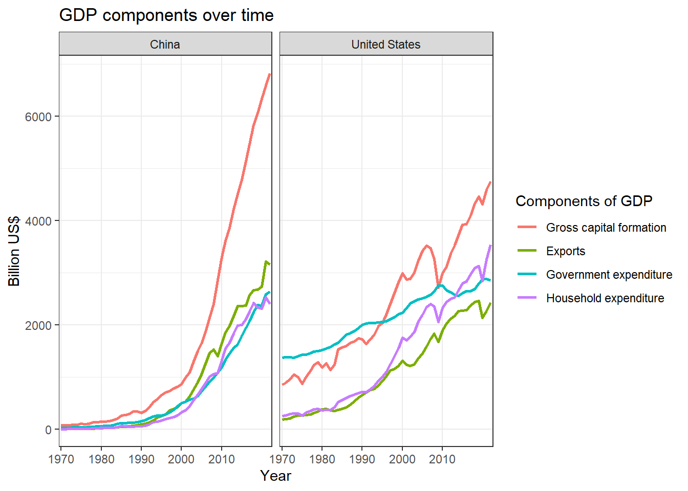
GDP components over time (China and the US)

Observation: It is evident that China’s GDP experienced a significant surge after the 1990s and continued to grow without reversal. The primary factor contributing to this growth was gross capital formation, which is closely related to the rise in manufacturing within the country.

Components as a Proportion of Total GDP

This analysis is centered on the calculation and visualization of the proportions of GDP components. By depicting each component as a fraction of the total GDP, we demonstrate how economic priorities change in relation to the overall economic output. Comparing these trends across different countries reveals variations in spending behaviors and economic structures, offering insights into long-term economic trends and the effects of policy decisions.

comp_wide <- dcast(comp, Country + Year ~ IndicatorName)

comp_wide$Net.Exports <- 
  comp_wide[, "Exports"] - comp_wide[, "Imports"]

comp2_wide <- 
  subset(comp_wide, select = -c(Exports, Imports))

comp2 <-
  melt(comp2_wide, id.vars = c("Year", "Country"))

props = comp2 %>%
  group_by(Country, Year) %>%
  mutate(proportion = value / sum(value))

Code Explanation:

This code snippet reshapes GDP data into wide format (comp_wide), calculates net exports, and then transforms the data back into long format (comp2). It creates a new dataframe props where each GDP component`s value is expressed as a proportion of total GDP for each country and year using the mutate function with the piping operator %>%. This process groups data by country and year, calculates each component`s proportion relative to the sum of all components in that group, and stores the results in props

pl = ggplot(props, aes(x = Year, y = proportion, 
  color = variable))

pl = pl + geom_line(aes(group = variable), 
  size = 1)

pl = pl + scale_x_discrete(breaks = seq(1970, 2016,
  by = 10))

pl = pl + ggtitle("GDP component proportions over time")

pl = pl + theme_bw()

pl = pl + facet_wrap(~Country)

pl = pl + scale_colour_discrete(
  name = "Components of GDP",
  labels = c("Gross capital formation",
    "Government expenditure",
    "Household expenditure", 
    "Net Exports"))

pl

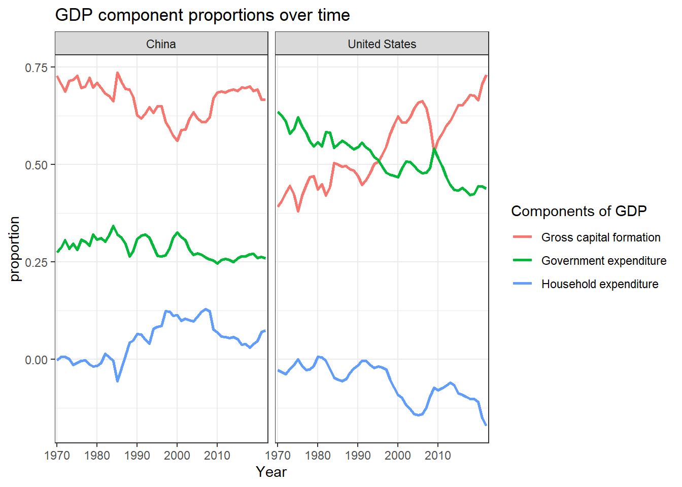
GDP component proportions over time (China and the US)

Observation: The graph illustrates the variations in the proportions of different components of the Gross Domestic Product (GDP) over the years.

pl = ggplot(props, aes(x = Year, y = proportion, 
  color = variable))

pl = pl + geom_line(aes(group = variable), 
  size = 1)

pl = pl + scale_x_discrete(breaks = seq(1970, 2016,
  by = 10))

pl = pl + ggtitle("GDP component proportions over time")

pl = pl + theme_bw()

pl = pl + facet_wrap(~Country)

pl = pl + scale_colour_discrete(
  name = "Components of GDP",
  labels = c("Gross capital formation",
    "Government expenditure",
    "Household expenditure", 
    "Net Exports"))

pl

Code Explanation:

This R code uses ggplot2 to create line charts for each country, showing how proportions of GDP components (like capital formation, government expenditure, etc.) have changed over time. Each line represents a GDP component, grouped by country, providing a clear visual comparison of economic priorities and trends across nations from 1970 to the present.

Charts using cross-sectional data⁠

Up to this point, we have conducted analyses of time series data, which consists of a collection of values for the same variables and subjects, recorded at different intervals (such as the annual GDP of a specific country). We will now proceed to create charts utilizing cross-sectional data, which encompasses values for the same variables across different subjects, typically collected simultaneously.

We choose the following countries for the analysis:

Developed countries: Germany, Japan, United States
Transition countries: Albania, Russian Federation, Ukraine
Developing countries: Brazil, China, India.

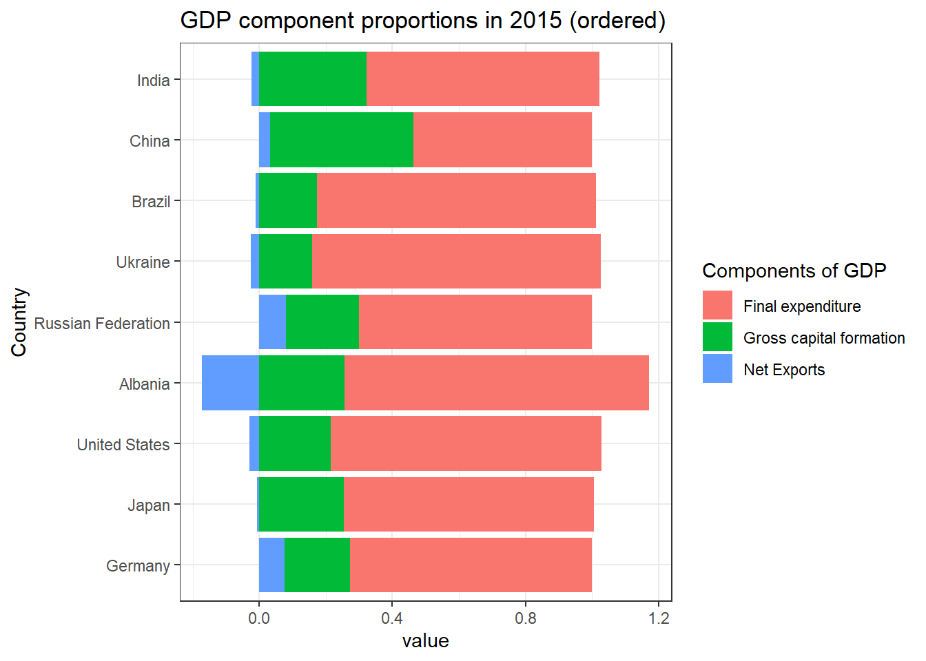
GDP component proportions in 2015

table_UN$p_Capital <- 
  table_UN$Capital / 
  (table_UN$Capital +
    table_UN$Final.Expenditure +
    table_UN$Net.Exports)

table_UN$p_FinalExp <-
  table_UN$Final.Expenditure / 
  (table_UN$Capital +
    table_UN$Final.Expenditure +
    table_UN$Net.Exports)

table_UN$p_NetExports <-
  table_UN$Net.Exports /
  (table_UN$Capital +
    table_UN$Final.Expenditure + 
    table_UN$Net.Exports)

sel_countries <- 
  c("Germany", "Japan", "United States",
    "Albania", "Russian Federation", "Ukraine",
    "Brazil", "China", "India")


sel_2015 <- 
  subset(table_UN, subset =
    (Country %in% sel_countries) & (Year == 2015),
    select = c("Country", "Year", "p_FinalExp",
      "p_Capital", "p_NetExports"))

sel_2015_m <- melt(sel_2015, id.vars = 
  c("Year", "Country"))

sel_2015_m$Country <- 
  factor(sel_2015_m$Country, levels = sel_countries)

g <- ggplot(sel_2015_m, 
  aes(x = Country, y = value, fill = variable)) +
  geom_bar(stat = "identity") + coord_flip() + 
  ggtitle("GDP component proportions in 2015 (ordered)") + 
  scale_fill_discrete(name = "Components of GDP", 
  labels = c("Final expenditure",
    "Gross capital formation",
    "Net Exports")) +
  theme_bw()

plot(g)

Code Explanation:

Calculating Proportions:

Computes proportions (p_Capital, p_FinalExp, p_NetExports) of GDP components relative to total GDP for each observation in table_UN.

Selecting Data:

Filters table_UN to include data for specific countries (sel_countries) and the year 2015 (sel_2015). Selects columns (Country, Year, p_FinalExp, p_Capital, p_NetExports) for analysis.

Plotting with ggplot2:

Uses ggplot2 to create a horizontal bar plot (geom_bar(stat = “identity”)) where each bar represents a GDP component`s proportion. Bars are grouped by country (Country) and colored by GDP component (variable).

1.3 GDP Per capita

Gross Domestic Product (GDP) per capita shows a country’s GDP divided by its total population. Gross domestic product (GDP) per capita is an economic metric that breaks down a country’s economic output to a per-person allocation.

GDP per capita is relatively simple to calculate and utilize. Furthermore, it serves as a fairly objective metric. It stands as the most commonly employed measure in economic analysis.

Even as a measure of material wellbeing, GDP per capita has limitations:

High levels of GDP per capita do not necessarily mean high levels of household disposable income, a key measure of average material well-being of people
Gross Domestic Product (GDP) per capita represents an average economic output per person within a nation, but it fails to account for disparities in material wellbeing among the population. Consequently, a nation can exhibit a high GDP per capita even if income is predominantly concentrated within a small segment of its populace.
It fails to account for non-market activities like volunteering, caregiving, and household work, which are important to people’s well-being.

2. HDI as a measure of material well-being

Why GDP is not a measure of Human Well-Being?

The critique of Gross Domestic Product (GDP) underscores its inadequacies in accurately representing societal well-being and environmental impact.

Although GDP quantifies economic output, it overlooks negative externalities such as pollution and health issues resulting from production activities. This omission results in distorted evaluations of development, particularly in instances where economic growth conceals environmental degradation.

Additionally, GDP does not consider income inequality or the transition towards service-oriented economies, diminishing its applicability in the contemporary context where quality of life and social equity are increasingly significant.

Consequently, there is a demand for alternative metrics that more effectively encapsulate overall welfare and sustainability in evaluating economic progress.

Human Development Index

We are now going to look at the Human Development Index (HDI), a measure of wellbeing that includes non-material aspects, and make comparisons with GDP per capita

The HDI consists of three dimensions associated with wellbeing:

a long and healthy life (health)
knowledge (education)
a decent standard of living (income).

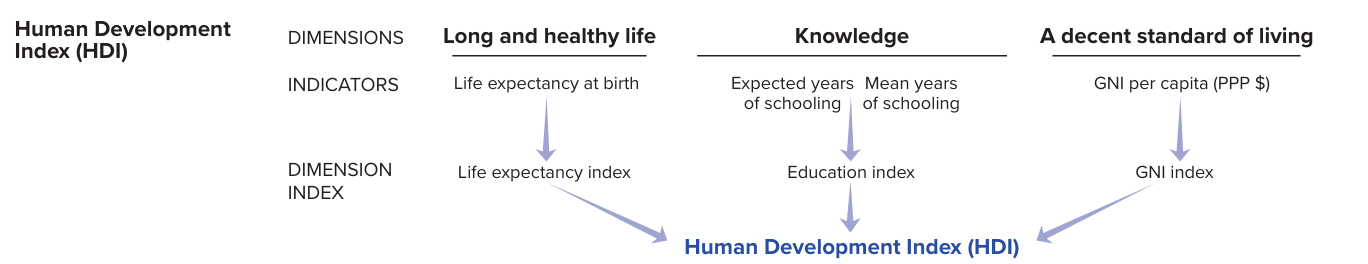
The HDI data we will look at is from the Human Development Report by the United Nations Development Programme (UNDP)

HDR2021 <- read_excel("HDI_Table.xlsx", sheet = "HDI", skip = 3)

## # A tibble: 6 × 15
##   ...1     ...2        Human Development In…¹ ...4  Life expectancy at b…² ...6 
##   <chr>    <chr>       <chr>                  <lgl> <chr>                  <chr>
## 1 HDI rank Country     Value                  NA    (years)                <NA> 
## 2 <NA>     <NA>        2022                   NA    2022                   <NA> 
## 3 <NA>     VERY HIGH … <NA>                   NA    <NA>                   <NA> 
## 4 1        Switzerland 0.96699999999999997    NA    84.254999999999995     <NA> 
## 5 2        Norway      0.96599999999999997    NA    83.393000000000001     <NA> 
## 6 3        Iceland     0.95899999999999996    NA    82.814999999999998     <NA> 
## # ℹ abbreviated names: ¹`Human Development Index (HDI)`,
## #   ²`Life expectancy at birth`
## # ℹ 9 more variables: `Expected years of schooling` <chr>, ...8 <chr>,
## #   `Mean years of schooling` <chr>, ...10 <chr>,
## #   `Gross national income (GNI) per capita` <chr>, ...12 <chr>,
## #   `GNI per capita rank minus HDI rank` <chr>, ...14 <chr>, `HDI rank` <chr>

Cleaning up the dataframe

The HDR dataframe contains non-data rows marked with ‘NA’ in the first column and columns starting with ‘…’ that lack meaningful information, except for columns labeled ‘…1’ (HDI rank) and ‘…2’ (country names). Hence we need to clean the data, to make it useful for proper analysis.

names(HDR2021)[1] <- "HDI.rank"

names(HDR2021)[2] <- "Country"

names(HDR2021)[names(HDR2021) == "HDI rank"] <- "HDI.rank.2020"

HDR2021 <- subset(HDR2021, !is.na(HDI.rank) & HDI.rank != "HDI rank")

sel_columns <- !startsWith(names(HDR2021), "...")
HDR2021 <- subset(HDR2021, select = sel_columns)

names(HDR2021)[3] <- "HDI"
names(HDR2021)[4] <- "LifeExp"
names(HDR2021)[5] <- "ExpSchool"
names(HDR2021)[6] <- "MeanSchool"
names(HDR2021)[7] <- "GNI.capita"
names(HDR2021)[8] <- "GNI.HDI.rank"

HDR2021$HDI.rank <- as.numeric(HDR2021$HDI.rank)
HDR2021$Country <- as.factor(HDR2021$Country)
HDR2021$HDI <- as.numeric(HDR2021$HDI)
HDR2021$LifeExp <- as.numeric(HDR2021$LifeExp)
HDR2021$ExpSchool <- as.numeric(HDR2021$ExpSchool)
HDR2021$MeanSchool <- as.numeric(HDR2021$MeanSchool)
HDR2021$GNI.capita <- as.numeric(HDR2021$GNI.capita)
HDR2021$GNI.HDI.rank <- as.numeric(HDR2021$GNI.HDI.rank)
HDR2021$HDI.rank.2020 <- as.numeric(HDR2021$HDI.rank.2020)

Code Explanation:

This code snippet prepares the HDR2021 dataframe by renaming columns for clarity, removing non-data rows, selecting relevant columns, and ensuring numeric data types are correctly assigned for analysis. It focuses on organizing the data for easier interpretation and statistical operations.

2.1 Calculating HDI

Dimension	Indicator	Minimum	Maximum
Health	Life Expectancy(years)	20	85
Education	Expected years of schooling (years)	0	18
Standard of Living	Gross National income per capita (2011 PPP $)	100	75000

United Nations Development Programme. 2022. ‘Technical notes’ in Human Development Report 2021/22: p. 2.

We will now recalculate HDI from its indicators.

The HDI indicators are measured in different units and have different ranges, so in order to put them together into a meaningful index, we need to normalize the indicators using the following formula:

Dimension index = (actual value - minimum value)(maximum value - minimum value)

HDR2021$I.Health <- 
  (HDR2021$LifeExp - 20) / (85 - 20)

HDR2021$I.Education <- 
  ((pmin(HDR2021$ExpSchool, 18) - 0) / 
  (18 - 0) + (HDR2021$MeanSchool - 0) / 
  (15 - 0)) / 2

HDR2021$I.Income <-
  (log(HDR2021$GNI.capita) - log(100)) /
  (log(75000) - log(100))

Code Explanation:

This code calculates components and a composite Human Development Index (HDI) for the HDR2021 dataframe:

I.Health: Normalizes life expectancy (LifeExp) between 20 and 85.
I.Education: Combines normalized Expected Years of Schooling (ExpSchool) and Mean Years of Schooling (MeanSchool).
I.Income: Normalizes Gross National Income per capita (GNI.capita) logarithmically between 100 and 75,000.

Now, we can combine these dimensional indices to give the HDI. The HDI is the geometric mean⁠ of the three dimension indices:

HDI = (I_{Health} * I_{Education} * I_{Income})^{1/3}

HDR2021$HDI.calc <- 
  (HDR2021$I.Health * HDR2021$I.Education * 
    HDR2021$I.Income)^(1/3)

We can now compare the HDI given in the table and our calculated HDI.

## # A tibble: 193 × 2
##      HDI HDI.calc
##    <dbl>    <dbl>
##  1 0.967    0.967
##  2 0.966    0.966
##  3 0.959    0.959
##  4 0.956    0.956
##  5 0.952    0.952
##  6 0.952    0.952
##  7 0.95     0.950
##  8 0.95     0.957
##  9 0.949    0.957
## 10 0.946    0.946
## # ℹ 183 more rows

Hence, we can see that the method of measuring HDI is correct, as the approximate values of calculated HDI match the HDI given in the table.

2.2 Creating own Index of Non-Material Wellbeing

We choose the following indicators for our index:

Immunization, measles (% of children ages 12-23 months)
Hospital beds (per 1,000 people)
Employment to population ratio, 15+, total (%) (national estimate)
Rule of Law: Percentile Rank
Voice and Accountability: Percentile Rank
Gross domestic savings (% of GDP)

The data for these indicators has been taken from Databank | World Bank{.uri}

## # A tibble: 6 × 66
##   `Country Name` `Series Name`  `1960` `1961` `1962` `1963` `1964` `1965` `1966`
##   <chr>          <chr>           <dbl>  <dbl>  <dbl>  <dbl>  <dbl>  <dbl>  <dbl>
## 1 Afghanistan    Immunization,… NA       NA     NA    NA     NA     NA     NA   
## 2 Afghanistan    Hospital beds…  0.171   NA     NA    NA     NA     NA     NA   
## 3 Afghanistan    Employment to… NA       NA     NA    NA     NA     NA     NA   
## 4 Afghanistan    Rule of Law: … NA       NA     NA    NA     NA     NA     NA   
## 5 Afghanistan    Voice and Acc… NA       NA     NA    NA     NA     NA     NA   
## 6 Afghanistan    Gross domesti… 13.2     13.0   14.6   6.51   4.72   1.10  -1.59
## # ℹ 57 more variables: `1967` <dbl>, `1968` <dbl>, `1969` <dbl>, `1970` <dbl>,
## #   `1971` <dbl>, `1972` <dbl>, `1973` <dbl>, `1974` <dbl>, `1975` <dbl>,
## #   `1976` <dbl>, `1977` <dbl>, `1978` <dbl>, `1979` <dbl>, `1980` <dbl>,
## #   `1981` <dbl>, `1982` <dbl>, `1983` <dbl>, `1984` <dbl>, `1985` <dbl>,
## #   `1986` <dbl>, `1987` <dbl>, `1988` <dbl>, `1989` <dbl>, `1990` <dbl>,
## #   `1991` <dbl>, `1992` <dbl>, `1993` <dbl>, `1994` <dbl>, `1995` <dbl>,
## #   `1996` <dbl>, `1997` <dbl>, `1998` <dbl>, `1999` <dbl>, `2000` <dbl>, …

Cleaning the Data

wide_indicator <- indicator_data

Created a replica of original data set for further analysis


id_vars <- c("Country Name", "Series Name")


long_indicator <- melt(wide_indicator, id.vars = id_vars, value.vars = 3:ncol(wide_indicator), variable.name = "Year", value.name = "Value")

long_indicator$`Series Name`[long_indicator$`Series Name`==
                               strwrap("Hospital beds (per 1,000 people)")] <- "I.HospitalBeds"

long_indicator$`Series Name` <- gsub("Employment to population ratio, 15\\+, total \\(\\%\\) \\(national estimate\\)", "I.EmploymentRatio", long_indicator$`Series Name`)

long_indicator$`Series Name` <- gsub("Immunization, measles \\(\\% of children ages 12-23 months\\)", "I.Immunization", long_indicator$`Series Name`)

long_indicator$`Series Name` <- gsub("Rule of Law: Percentile Rank", "I.RuleofLaw", long_indicator$`Series Name`)
long_indicator$`Series Name` <- gsub("Voice and Accountability: Percentile Rank", "I.Voice", long_indicator$`Series Name`)

long_indicator$`Series Name`[long_indicator$`Series Name`==
                               strwrap("Gross domestic savings (% of GDP)")] <- "I.GDS"


colnames(long_indicator) <- c("country","indicator","year", "value")

converted wide_indicator to long form.

table_indicator <- pivot_wider(
  data = long_indicator,
  names_from = indicator,
  values_from = value
)

Converted again to wide form so that the format of the data becomes like given below-

## # A tibble: 6 × 9
##   country      year  I.Immunization I.HospitalBeds I.EmploymentRatio I.RuleofLaw
##   <chr>        <fct> <list>         <list>         <list>            <list>     
## 1 Afghanistan  1960  <dbl [1]>      <dbl [1]>      <dbl [1]>         <dbl [1]>  
## 2 Albania      1960  <dbl [1]>      <dbl [1]>      <dbl [1]>         <dbl [1]>  
## 3 Algeria      1960  <dbl [1]>      <dbl [1]>      <dbl [1]>         <dbl [1]>  
## 4 American Sa… 1960  <dbl [1]>      <dbl [1]>      <dbl [1]>         <dbl [1]>  
## 5 Andorra      1960  <dbl [1]>      <dbl [1]>      <dbl [1]>         <dbl [1]>  
## 6 Angola       1960  <dbl [1]>      <dbl [1]>      <dbl [1]>         <dbl [1]>  
## # ℹ 3 more variables: I.Voice <list>, I.GDS <list>, `NA` <list>

HDN <- subset(table_indicator, year == '2019')
HDN <- HDN[,-9]

created a subset HDN for year 2019


HDN_df = as.data.frame(HDN)


HDN_check <- HDN_df %>% 
  mutate(country, country == "NA", NA) %>%
  mutate(year, year == "NA", NA) %>%
  mutate(I.Immunization, I.Immunization == "NA", NA) %>% 
  mutate(I.HospitalBeds, I.HospitalBeds == "NA", NA) %>%
  mutate(I.EmploymentRatio, I.EmploymentRatio == "NA", NA) %>%
  mutate(I.RuleofLaw, I.RuleofLaw == "NA", NA) %>%
  mutate(I.Voice, I.Voice == "NA", NA) %>%
  mutate(I.GDS, I.GDS == "NA", NA)

HDN_check <- HDN_check[,-10]
  

HDN_logical <- HDN_check[,9:16] 

HDN_filtered <- HDN_df[!apply(HDN_logical, 1, any), ]

created a logical df HDN_logical which has TRUE where values NA, and then creating HDN_filtered containing only those countries that have values of all the indicators.



HDN2019 <- HDN_filtered %>%
  unnest(cols = c(I.Immunization, I.HospitalBeds, I.EmploymentRatio, 
                  I.RuleofLaw, I.Voice, I.GDS)) %>%
  mutate(
    I.Immunization = as.numeric(I.Immunization),
    I.HospitalBeds = as.numeric(I.HospitalBeds),
    I.EmploymentRatio = as.numeric(I.EmploymentRatio),
    I.RuleofLaw = as.numeric(I.RuleofLaw),
    I.Voice = as.numeric(I.Voice),
    I.GDS = as.numeric(I.GDS)
  )
summary(HDN2019)

converting the type of values from “character” to “numeric”

HDN2019$I.ImmunizationC <- (HDN2019$I.Immunization - 90)/(99-90)

HDN2019$I.HospitalBedsC <- (HDN2019$I.HospitalBeds - 1.1)/(5.8-1.1)

HDN2019$I.EmploymentRatioC <- (HDN2019$I.EmploymentRatio - 51.475)/(78.39-51.475)

HDN2019$I.RuleofLawC <- (HDN2019$I.RuleofLaw - 70)/(98-70)

HDN2019$I.VoiceC <- (HDN2019$I.Voice - 84.06)/(98.55-84.06)

HDN2019$I.GDSC <- (HDN2019$I.GDS - 16.98310)/(16.98310-49.17)

HDN2019$HDI.calc <- (HDN2019$I.ImmunizationC * HDN2019$I.HospitalBedsC *  HDN2019$I.EmploymentRatioC * HDN2019$I.RuleofLawC * HDN2019$I.VoiceC * HDN2019$I.GDSC)^(1/6)

Here are the results:-

HDN2019$HDI.calc

And here are the various indices:

HDN2019$I.ImmunizationC
HDN2019$I.HospitalBedsC
HDN2019$I.EmploymentRatioC
HDN2019$I.RuleofLawC
HDN2019$I.VoiceC
HDN2019$I.GDSC