Measuring Willingness to Pay for Climate Change Abatement
As businesses shift towards pursuing environmental, social, and governance (ESG) means, abatement costs play a large role in discouraging companies from leniency on their environmental greenhouse gas emissions.
Specifically, abatement costs are there as “fines” for companies that either fail to innovate in creating greener production cycles or fail to account for potential problems and end up damaging the environment.
Abatement Costs
The most common scenario in which abatement costs are applied is for pollution and oil spills, whether accidental or intentional.
In this project, as an illustrative example, we will examine climate change mitigation. Addressing climate change often involves short-term expenses, such as the reforestation of degraded forests.
Consequently, governments may seek to understand the extent to which their citizens are willing to financially contribute towards reducing carbon emissions as a strategy for mitigating climate change.
1. Summarizing the Data
We will be using data collected from an internet survey sponsored by the German government.
Two common ways of obtaining information about willingness to pay (WTP) are:
-
dichotomous choice (DC): presenting individuals with an amount, to which they respond with either ‘yes/willing to pay’ or ‘no/not willing to pay’ (sometimes a ‘no response’ option is also offered)
-
a two-way payment ladder (TWPL): asking individuals to state the minimum and maximum amount they are willing to pay (selecting from a pre-specified list of amounts).
The German government sponsored a nationwide online survey that investigated the effect of question format (DC or TWPL) on WTP responses.
WTP <- read_excel("excel-project-11.xlsx", sheet = "Data")Code Explanation:
This code imports the dataset into the project for further analysis.
Reverse-coding variables
Attitudes were evaluated utilizing a Likert scale ranging from 1 to 5, with 1 representing strong disagreement and 5 representing strong agreement.
The phrasing of the questions varied, resulting in an answer of ‘strongly agree’ indicating high climate change skepticism for one question and low skepticism for another. To consolidate these questions into a single index, it is necessary to recode, specifically reverse-code, certain variables.
We will reverse the following variables:
-
cog_2 -
cog_5 -
scepticism_6 -
scepticism_7
WTP <- WTP %>%
  mutate_at(c("cog_2", "cog_5",
    "scepticism_6", "scepticism_7"),
    funs(recode(., "1" = 5, "2" = 4, "3" = 3,
      "4" = 2, "5" = 1)))
Code Explanation:
This R code uses the dplyr package to transform (mutate) specific columns (cog_2, cog_5, scepticism_6, scepticism_7) in the dataframe WTP. It recodes values "1" to 5, "2" to 4, "3" to 3, "4" to 2, and "5" to 1 in these columns, effectively swapping their numeric values in a descending order.
Creating some new variables
For the variables WTP_plmin and WTP_plmax, create new variables with the values replaced with the actual euro values.
wtp_euro_levels <- c(48, 72, 84, 108, 156, 192, 252, 324,
  432, 540, 720, 960, 1200, 1440)

category_amount <- data.frame(original = 1:14,
  new = wtp_euro_levels)

WTP <- merge(WTP, category_amount,
  by.x = "WTP_plmin", by.y = "original",
  all.x = TRUE) %>%
  rename(., "WTP_plmin_euro" = "new")

WTP <- merge(WTP, category_amount,
  by.x = "WTP_plmax", by.y = "original", all.x = TRUE) %>%
  rename(., "WTP_plmax_euro" = "new")
Code Explanation:
The code defines a vector wtp_euro_levels containing specified euro amounts. It then creates a dataframe category_amount with columns original (ranging from 1 to 14) and new (mapped to wtp_euro_levels).
The dataframe WTP is merged twice with category_amount based on columns WTP_plmin and WTP_plmax. After each merge, the merged column (new from category_amount) is renamed to WTP_plmin_euro and WTP_plmax_euro, respectively.
These operations effectively map specific euro amounts to corresponding values in WTP based on WTP_plmin and WTP_plmax columns.
Creating Indices
We create three new indices:
-
climate: Belief that climate change is a real phenomenon -
gov_intervention: Preferences for government intervention to solve problems in society -
pro_environment: Feeling of personal responsibility to act pro-environmentally
creating indices
WTP <- WTP %>%

  rowwise() %>%
  mutate(., climate = rowMeans(cbind(
    scepticism_2, scepticism_6, scepticism_7))) %>%
  mutate(., gov_intervention = rowMeans(cbind(
    cog_1, cog_2, cog_3, cog_4, cog_5, cog_6))) %>%
  mutate(., pro_environment  = rowMeans(cbind(
    PN_1, PN_2, PN_3, PN_4, PN_6, PN_7))) %>%
  ungroup()
Assessing Consistency/Reliability
There are two prevalent methods to evaluate reliability: one involves examining the correlation between items within the index, and the other employs a summary measure known as Cronbach’s alpha.
Cronbach’s alpha is a way to summarize the correlations between many variables, and ranges from 0 to 1, with 0 meaning that all of the items are independent of one another, and 1 meaning that all of the items are perfectly correlated with each other. While higher values of this measure indicate that the items are closely related and therefore measure the same concept, with values that are very close to 1 (or 1), we could be concerned that our index contains redundant items
Cronbach’s alpha is computed by correlating the score for each scale item with the total score for each observation (usually individual survey respondents or test takers), and then comparing that to the variance for all individual item scores:
$$ \alpha = (\frac{k}{k - 1})(1 - \frac{\sum_{i=1}^{k} \sigma_{y_{i}}^{2}}{\sigma_{x}^{2}}) $$
where:
-
k refers to number of scale items
-
$\sigma_{y_{i}}^2$ refers to the variance associated with item i
-
$\sigma_{x}^2$ refers to the variance associated with the observed total scores
Calculating Correlation Coefficients:
- For questions on climate change
cor(cbind(WTP$scepticism_2, WTP$scepticism_6,
  WTP$scepticism_7))
## exaggeration not.human.activity no.evidence
## exaggeration 1.0000000 0.3904296 0.4167478
## not.human.activity 0.3904296 1.0000000 0.4624211
## no.evidence 0.4167478 0.4624211 1.0000000Correlation table for survey items on climate change scepticism: Climate change is exaggerated (exaggeration), Human activity is not the main cause of climate change (not.human.activity), No evidence of global warming (no.evidence)
- For questions on government behavior :
cor(cbind(WTP$cog_1, WTP$cog_2, WTP$cog_3,
  WTP$cog_4, WTP$cog_5, WTP$cog_6))
## too.much not.pass.laws minimal.intervention
## too.much 1.0000000 0.2509464 0.32358783
## not.pass.laws 0.2509464 1.0000000 0.11761093
## minimal.intervention 0.3235878 0.1176109 1.00000000
## not.dictate 0.6823385 0.2771883 0.33476619
## indiv.freedom 0.2892567 0.4079467 0.01818617
## personal.responsibility 0.4141992 0.0828661 0.31286082
## not.dictate indiv.freedom personal.responsibility
## too.much 0.6823385 0.28925672 0.4141992
## not.pass.laws 0.2771883 0.40794667 0.0828661
## minimal.intervention 0.3347662 0.01818617 0.3128608
## not.dictate 1.0000000 0.27424993 0.4597244
## indiv.freedom 0.2742499 1.00000000 0.1045843
## personal.responsibility 0.4597244 0.10458434 1.0000000Table displaying the correlation among survey questions regarding government involvement: excessive government interference (too.much), opposition to government legislation enabling individuals to act in their own interest (not.pass.laws), preference for minimal government intervention in economic affairs (minimal.intervention), disapproval of government imposition on personal lifestyle choices (not.dictate), reluctance for the government to prioritize social objectives over individual liberties (indiv.freedom), advocacy for increased personal accountability among individuals (personal.responsibility).
- For questions on personal behavior :
cor(cbind(WTP$PN_1, WTP$PN_2, WTP$PN_3,
  WTP$PN_4, WTP$PN_6, WTP$PN_7))
## buy.local indiv.impact feel.better public.transport
## buy.local 1.0000000 0.4824823 0.4282149 0.4226534
## indiv.impact 0.4824823 1.0000000 0.6315015 0.4375971
## feel.better 0.4282149 0.6315015 1.0000000 0.4596711
## public.transport 0.4226534 0.4375971 0.4596711 1.0000000
## conserve.energy 0.4138090 0.4994126 0.5219712 0.5668642
## reduce.emissions 0.4584007 0.6542377 0.5894731 0.3947270
## conserve.energy reduce.emissions
## buy.local 0.4138090 0.4584007
## indiv.impact 0.4994126 0.6542377
## feel.better 0.5219712 0.5894731
## public.transport 0.5668642 0.3947270
## conserve.energy 1.0000000 0.4551294
## reduce.emissions 0.4551294 1.0000000Correlation table for survey items on ‘personal responsibility for the environment’: I buy locally to reduce emissions (buy.local), I am obliged to take impact of daily activities on climate (individual.impact), I feel better when reducing emissions (feel.better), I prefer to use public transport (public.transport), I feel uncomfortable when consuming energy (conserve.energy), I try to reduce emissions as much as possible (reduce.emissions).
Calculating Cronbach’s Alpha:
We use the aplha function from the psych package to calculate Cronbach’s Alpha.
psych::alpha(WTP[c("scepticism_2",
  "scepticism_6", "scepticism_7")])$total$std.alpha

psych::alpha(WTP[c("cog_1", "cog_2", "cog_3",
  "cog_4", "cog_5", "cog_6")])$total$std.alpha

psych::alpha(WTP[c("PN_1", "PN_2", "PN_3",
  "PN_4", "PN_6", "PN_7")])$total$std.alpha
## [1] 0.6876079
## [1] 0.7102249
## [1] 0.8543827Code Explanation:
These R commands are utilized to compute Cronbach`s alpha for various sets of variables—namely scepticism, cognitive, and PN—within the dataframe WTP, employing the psych package.
The coefficient values in question are high, suggesting that the indicators within each category measure the same underlying concept.
1.1 Comparing characteristics of people in DC group and TWPL group
For each group, we compare them on the following basis:
-
gender (
sex) -
age (
age) -
number of children (
kids_nr) -
household net income per month in euros (
hhnetinc) -
membership in environmental organization (
member) -
highest educational attainment (
education)
variables <- list(quo(sex), quo(age),
  quo(kids_nr), quo(hhnetinc),
  quo(member), quo(education))

result_list <- list()

for (i in seq_along(variables)) {
  result <- WTP %>%
    group_by(abst_format, !!variables[[i]]) %>%
    summarize(n = n()) %>%
    mutate(freq = n / sum(n) * 100) %>%  # Calculate percentage
    select(-n) %>%
    spread(abst_format, freq) %>%
    rename(TWPL = 'ladder', DC = 'ref')  # Rename columns

  result_list[[i]] <- result
}

print(result_list)
## [[1]]
## # A tibble: 2 × 3
## sex TWPL DC
## <chr> <dbl> <dbl>
## 1 female 51.8 52.3
## 2 male 48.2 47.7
##
## [[2]]
## # A tibble: 6 × 3
## age TWPL DC
## <chr> <dbl> <dbl>
## 1 18 - 24 9.49 9.64
## 2 25 - 29 8.30 8.65
## 3 30 - 39 17.8 17.2
## 4 40 - 49 22.3 22.6
## 5 50 - 59 24.1 23.9
## 6 60 - 69 18.0 18.1
##
## [[3]]
## # A tibble: 5 × 3
## kids_nr TWPL DC
## <chr> <dbl> <dbl>
## 1 four or more children 0.988 0.895
## 2 no children 64.6 65.7
## 3 one child 20.4 17.6
## 4 three children 2.96 3.48
## 5 two children 11.1 12.3
##
## [[4]]
## # A tibble: 12 × 3
## hhnetinc TWPL DC
## <chr> <dbl> <dbl>
## 1 1100 bis unter 1500 Euro 14.2 13.2
## 2 1500 bis unter 2000 Euro 15.0 14.6
## 3 2000 bis unter 2600 Euro 11.5 14.8
## 4 2600 bis unter 3200 Euro 10.7 10.7
## 5 3200 bis unter 4000 Euro 11.1 8.15
## 6 4000 bis unter 5000 Euro 5.14 4.97
## 7 500 bis unter 1100 Euro 13.4 14.2
## 8 5000 bis unter 6000 Euro 2.77 1.69
## 9 6000 bis unter 7500 Euro 0.791 0.398
## 10 7500 und mehr 0.395 0.497
## 11 bis unter 500 Euro 2.96 4.17
## 12 do not want to answer 12.1 12.5
##
## [[5]]
## # A tibble: 2 × 3
## member TWPL DC
## <chr> <dbl> <dbl>
## 1 no 92.3 91.4
## 2 yes 7.71 8.65
##
## [[6]]
## # A tibble: 6 × 3
## education TWPL DC
## <dbl> <dbl> <dbl>
## 1 1 1.19 1.29
## 2 2 1.98 2.09
## 3 3 34.2 32.8
## 4 4 26.3 26.9
## 5 5 6.92 6.86
## 6 6 29.4 30.0Code Explanation:
This R code iterates through categorical variables (sex, age, kids_nr, hhnetinc, member, education) in the WTP dataframe. For each variable, it groups data by abst_format, calculates frequencies (freq) based on counts (n), removes the count column, and spreads the results into wide-format tables. This analysis helps understand how each variable distributes across different abst_format categories.
WTP %>%
  group_by(abst_format) %>%
  summarise_at(c("climate", "gov_intervention",
      "pro_environment"),
    funs(mean, sd, min, max)) %>%

  gather(index, value,
    climate_mean:pro_environment_max) %>%
  spread(abst_format, value) %>%
  rename(TWPL = 'ladder', DC = 'ref') %>%
kable(., format = "markdown", digits = 2)| index | TWPL | DC |
|---|---|---|
| climate_max | 5.00 | 5.00 |
| climate_mean | 2.29 | 2.37 |
| climate_min | 1.00 | 1.00 |
| climate_sd | 0.84 | 0.85 |
| gov_intervention_max | 5.00 | 5.00 |
| gov_intervention_mean | 3.15 | 3.19 |
| gov_intervention_min | 1.00 | 1.00 |
| gov_intervention_sd | 0.70 | 0.66 |
| pro_environment_max | 5.00 | 5.00 |
| pro_environment_mean | 3.03 | 3.01 |
| pro_environment_min | 1.00 | 1.00 |
| pro_environment_sd | 0.79 | 0.82 |
Observation:
The two groups are quite similar in attitudes. We can be reasonably confident that any differences in survey responses is due to the question format rather than differences in attitudes or demographics.
2. Comparing Willingness to pay across methods and individual characteristics
We begin this analysis by summarizing the distribution of WTP within each question format. We use the following column charts for this analysis.
For minimum willingness to pay:
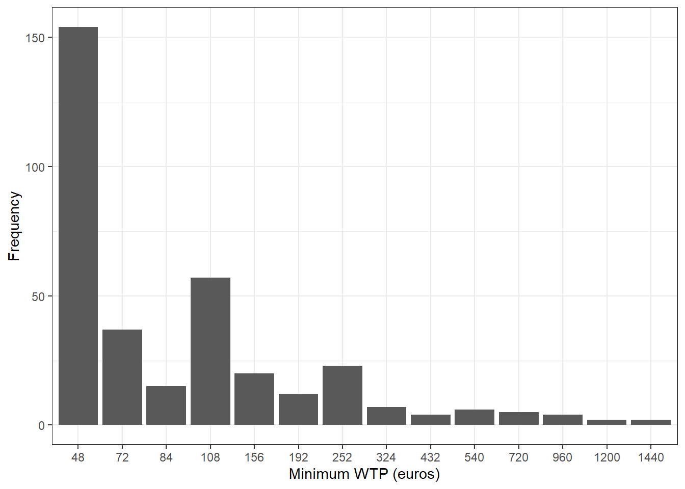
Observation: We can observe that a majority of people have the price of 48 euros as the price they would definitely vote in favor of.
For the maximum willingness to pay:
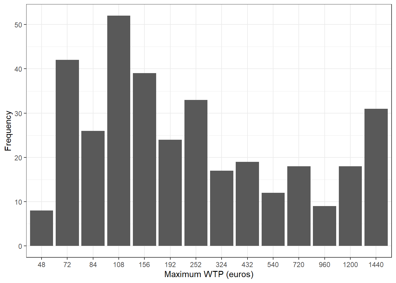
Observation: Despite the broad range in the maximum price at which individuals would cease to support, it is evident that 108 euros is the price most frequently selected by the majority.
df.plmax <- WTP %>%
  select(WTP_plmax_euro) %>%
  na.omit() %>%
  group_by(WTP_plmax_euro) %>%
  summarize(n = n()) %>%
  mutate(WTP_plmax_euro = factor(WTP_plmax_euro,
    levels = wtp_euro_levels))

ggplot(df.plmax, aes(WTP_plmax_euro, n)) +
  geom_bar(stat = "identity", position = "identity") +
  xlab("Maximum WTP (euros)") +
  ylab("Frequency") +
  theme_bw()
::: {style=“border: 1px solid black; padding: 10px; background-color: #f0f0f0; margin-bottom: 10px;”}
Code Explanation:
This R code uses **`ggplot2`** to create a bar plot showing how maximum willingness-to-pay **(`WTP_plmax_euro`)** values are distributed across predefined euro levels in the `WTP` data-set. It calculates frequencies for each **`WTP_plmax_euro`** value after grouping and converts it into a factor with specified levels. The plot displays frequencies on the y-axis and **`WTP_plmax_euro`** values on the x-axis, with a black and white theme for clarity.
:::Calculating average WTP for each individual
WTP <- WTP %>%
  rowwise() %>%
  mutate(., WTP_average = rowMeans(cbind(
    WTP_plmin_euro, WTP_plmax_euro))) %>%
  ungroup()
::: {style=“border: 1px solid black; padding: 10px; background-color: #f0f0f0; margin-bottom: 10px;”}
Code Explanation:
This code calculates the row-wise average of two existing columns (**`WTP_plmin_euro`** and **`WTP_plmax_euro`**) in the `WTP` data frame and stores the result in a new column named **`WTP_average`**.
:::mean(WTP$WTP_average, na.rm = TRUE)
median(WTP$WTP_average, na.rm = TRUE)## [1] 268.5345
## [2] 132The above given are the values of mean and median of this average value variable created by us.
Calculating correlation coefficients
WTP %>%
  mutate(gender =
    as.numeric(ifelse(sex == "female", 0, 1))) %>%
  select(WTP_average, education, gender,
    climate, gov_intervention, pro_environment) %>%
  cor(., use = "pairwise.complete.obs") -> M

M[, "WTP_average"]
::: {style=“border: 1px solid black; padding: 10px; background-color: #f0f0f0; margin-bottom: 10px;”}
Code Explanation:
This code calculates the correlation between **`WTP_average`** (presumably a derived column from a previous operation) and several other selected variables (*`education`*, *`gender`*, *`climate`*, *`gov_intervention`*, *`pro_environment`*) in the `WTP` data frame. It first converts the `sex` column to numeric values in the `gender` column and then computes the correlation matrix using complete observations, storing the result in `M`. Finally, it extracts and likely inspects the correlations involving `WTP_average`.
:::Observation:
-
WTP_averagewitheducation:-
Correlation coefficient of 0.13817368.
-
Indicates a weak positive correlation between
WTP_averageandeducation
-
-
WTP_averagewithgender:-
Correlation coefficient of 0.03694972.
-
Indicates a very weak positive correlation between
WTP_averageandgender
-
-
WTP_averagewithclimate:-
Correlation coefficient of -0.14462072.
-
Indicates a moderate negative correlation between
WTP_averageandclimate. This means as concerns or perceptions related to climate increase, the average willingness to pay (WTP_average) tends to decrease.
-
-
WTP_averagewithgov_intervention:-
Correlation coefficient of -0.18845205.
-
Indicates a moderate negative correlation between
WTP_averageandgov_intervention. This suggests that as support or favorability towards government intervention increases, the average willingness to pay (WTP_average) tends to decrease.
-
-
WTP_averagewithpro_environment:-
Correlation coefficient of 0.18750331.
-
Indicates a moderate positive correlation between
WTP_averageandpro_environment.
-
2.1 Comparing question formats
For individuals who answered DC(dichotomous choice) questions
Each individual was given an amount and had to decide ‘yes’, ‘no’, or ‘no vote/abstain from deciding’.
| costs | Abstain | No | Yes |
|---|---|---|---|
| 48 | 12 | 21 | 32 |
| 72 | 11 | 30 | 40 |
| 84 | 12 | 24 | 45 |
| 108 | 7 | 35 | 31 |
| 156 | 13 | 31 | 40 |
| 192 | 11 | 25 | 25 |
| 252 | 9 | 32 | 28 |
| 324 | 16 | 41 | 27 |
| 432 | 11 | 35 | 29 |
| 540 | 9 | 31 | 22 |
| 720 | 12 | 39 | 13 |
| 960 | 14 | 28 | 15 |
| 1200 | 11 | 42 | 21 |
| 1440 | 19 | 42 | 15 |
This table illustrates the distribution of individuals according to their voting choices and the associated costs.
WTP_DC <- WTP %>%
  group_by(costs, DC_ref_outcome) %>%
  summarize(n = n()) %>%
  na.omit() %>%
  mutate_at("DC_ref_outcome",
    funs(recode(.,
      "do not support referendum and no pay" = "No",
      "support referendum and pay" = "Yes",
      "would not vote" = "Abstain"))) %>%
  spread(DC_ref_outcome, n)

kable(WTP_DC, format = "markdown", digits = 2)
::: {style=“border: 1px solid black; padding: 10px; background-color: #f0f0f0; margin-bottom: 10px;”}
Code Explanation:
The code groups the `WTP` data by `costs` and `DC_ref_outcome`, counts the number of observations for each group, removes any rows with missing values, and then recategorizes specific values in `DC_ref_outcome` before spreading the summarized data into a table format suitable for Markdown output.
:::Modifying the table to include proportions
| costs | Abstain | No | Yes | total | prop_no | prop_yes |
|---|---|---|---|---|---|---|
| 48 | 12 | 21 | 32 | 65 | 0.51 | 0.49 |
| 72 | 11 | 30 | 40 | 81 | 0.51 | 0.49 |
| 84 | 12 | 24 | 45 | 81 | 0.44 | 0.56 |
| 108 | 7 | 35 | 31 | 73 | 0.58 | 0.42 |
| 156 | 13 | 31 | 40 | 84 | 0.52 | 0.48 |
| 192 | 11 | 25 | 25 | 61 | 0.59 | 0.41 |
| 252 | 9 | 32 | 28 | 69 | 0.59 | 0.41 |
| 324 | 16 | 41 | 27 | 84 | 0.68 | 0.32 |
| 432 | 11 | 35 | 29 | 75 | 0.61 | 0.39 |
| 540 | 9 | 31 | 22 | 62 | 0.65 | 0.35 |
| 720 | 12 | 39 | 13 | 64 | 0.80 | 0.20 |
| 960 | 14 | 28 | 15 | 57 | 0.74 | 0.26 |
| 1200 | 11 | 42 | 21 | 74 | 0.72 | 0.28 |
| 1440 | 19 | 42 | 15 | 76 | 0.80 | 0.20 |
At this point, in addition to the numerical counts, we can observe the proportion of votes allocated to each option.
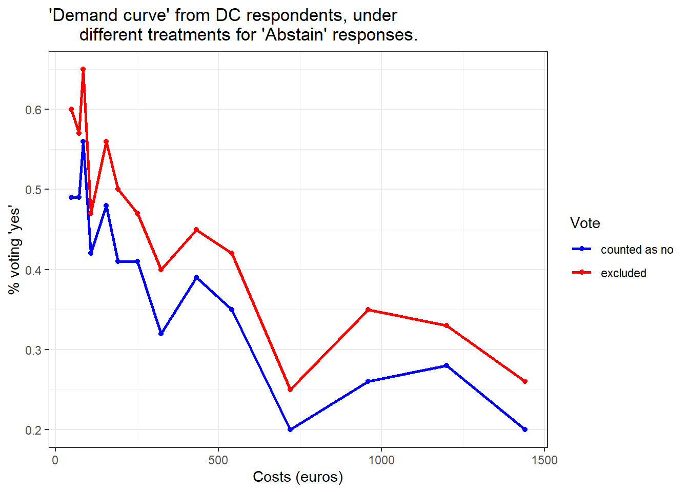
Visualizing WTP on a Demand Curve
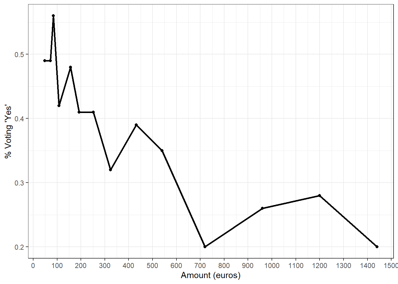
The demand curve typically exhibits a downward slope, indicating that the proportion of individuals voting ‘yes’ tends to diminish as the monetary amount rises.
Doing the analysis excluding individuals who chose 'abstain
| costs | Abstain | No | Yes | total | prop_no | prop_yes | total_ex | prop_no_ex | prop_yes_ex |
|---|---|---|---|---|---|---|---|---|---|
| 48 | 12 | 21 | 32 | 65 | 0.51 | 0.49 | 53 | 0.40 | 0.60 |
| 72 | 11 | 30 | 40 | 81 | 0.51 | 0.49 | 70 | 0.43 | 0.57 |
| 84 | 12 | 24 | 45 | 81 | 0.44 | 0.56 | 69 | 0.35 | 0.65 |
| 108 | 7 | 35 | 31 | 73 | 0.58 | 0.42 | 66 | 0.53 | 0.47 |
| 156 | 13 | 31 | 40 | 84 | 0.52 | 0.48 | 71 | 0.44 | 0.56 |
| 192 | 11 | 25 | 25 | 61 | 0.59 | 0.41 | 50 | 0.50 | 0.50 |
| 252 | 9 | 32 | 28 | 69 | 0.59 | 0.41 | 60 | 0.53 | 0.47 |
| 324 | 16 | 41 | 27 | 84 | 0.68 | 0.32 | 68 | 0.60 | 0.40 |
| 432 | 11 | 35 | 29 | 75 | 0.61 | 0.39 | 64 | 0.55 | 0.45 |
| 540 | 9 | 31 | 22 | 62 | 0.65 | 0.35 | 53 | 0.58 | 0.42 |
| 720 | 12 | 39 | 13 | 64 | 0.80 | 0.20 | 52 | 0.75 | 0.25 |
| 960 | 14 | 28 | 15 | 57 | 0.74 | 0.26 | 43 | 0.65 | 0.35 |
| 1200 | 11 | 42 | 21 | 74 | 0.72 | 0.28 | 63 | 0.67 | 0.33 |
| 1440 | 19 | 42 | 15 | 76 | 0.80 | 0.20 | 57 | 0.74 | 0.26 |
This table establishes new proportions for individuals who have participated in voting, excluding those who have chosen to abstain.
Comparing DC and TWPL question formats
For the DC format, willingness to pay is recorded in the costs variable, so we select all observations where the DC_ref_outcome variable indicates the individual voted ‘yes’ and drop any missing observations. For the TWPL format we use the WTP_average variable that we created.
Difference in means, standard deviations and number of observations
DC_WTP <- WTP %>% subset(
  DC_ref_outcome == "support referendum and pay") %>%
  select(costs) %>%
  filter(!is.na(costs)) %>%
  as.matrix()

TWPL_WTP <- WTP %>%
  select(WTP_average) %>%
  filter(!is.na(WTP_average)) %>%
  as.matrix()
::: {style=“border: 1px solid black; padding: 10px; background-color: #f0f0f0; margin-bottom: 10px;”}
Code Explanation:
The code first extracts a subset **`DC_WTP`** from the `WTP` data frame, containing only the **`costs`** values where **`DC_ref_outcome`** is "support referendum and pay". It ensures no missing values are included. Then, it creates **`TWPL_WTP`** by extracting non-missing `WTP_average` values from `WTP` and converts both subsets into matrices for further analysis.
:::cat(sprintf("DC Format -> mean: %.1f,
standard deviation %.1f, count %d\n",
mean(DC_WTP), sd(DC_WTP), length((DC_WTP))))cat(sprintf("TWPL Format -> mean: %.1f,
standard deviation %.1f, count %d\n",
mean(TWPL_WTP), sd(TWPL_WTP),
length((TWPL_WTP))))## DC Format -> mean: 348.2,
## standard deviation 378.6, count 383## TWPL Format -> mean: 268.5,
## standard deviation 287.7, count 348These statistics elucidate the variation in WTP values between the two survey formats. The mean values represent the average amount respondents are willing to pay under each format, while the standard deviations measure the variability in WTP responses. The counts reflect the number of valid responses used for each calculation, ensuring the reliability and representativeness of the findings for each survey method. Comparing these metrics aids in determining whether different survey formats elicit significantly different WTP responses from respondents.
95% Confidence Intervals
A confidence interval, in statistics, refers to the probability that a population parameter will fall between a set of values for a certain proportion of times. Thus, if a point estimate is generated from a statistical model of 10.00 with a 95% confidence interval of 9.50 to 10.50, it means one is 95% confident that the true value falls within that range.
A 95% confidence interval is a range of possible values within which the true value might lie. It is estimated from the mean and standard deviation of the data.
As the name suggests, confidence intervals tell us how much confidence we can place in our estimates, or in other words, how precisely the sample mean is estimated. The confidence interval gives us a margin of error for our estimate of the true value.
t.test(DC_WTP, TWPL_WTP, conf.level = 0.05)$conf.int## [1] 78.10141 81.20560
## attr(,"conf.level")
## [1] 0.05The ‘width’ of the confidence interval is 1.55, so the confidence interval is [79.65 – 1.55, 79.65 + 1.55], which is [78.10, 81.21].
The substantial difference in means (approximately 80 euros) is precisely estimated, indicating that the observed disparity is unlikely due to chance. Therefore, willingness to pay (WTP) is higher under the dichotomous choice (DC) format compared to the two-way payment ladder (TWPL) format.
3. Meeting the Paris Agreement Targets
Paris Agreement
The Paris Agreement is a legally binding international treaty on climate change. It was adopted by 196 Parties at the UN Climate Change Conference (COP21) in Paris, France, on 12 December 2015. It entered into force on 4 November 2016.
Its overarching goal is to hold “the increase in the global average temperature to well below 2°C above pre-industrial levels” and pursue efforts “to limit the temperature increase to 1.5°C above pre-industrial levels.”
3.1 Investment needed to achieve Paris Agreement Targets
For analyzing the investment needed to achieve Paris Agreement Targets, we will use Climate Investment Potential ($ billion) data given in the report Climate Investment Opportunities in Emerging Markets: An IFC Analysis
invst <- read_excel("climate investment oppurtunites-ifc-climate.xlsx")The data looks something like this:
## # A tibble: 6 × 12
##   `(in billions)`   Wind Solar Biomass `Small Hydro` Geothermal `All Renewables`
##   <chr>            <dbl> <dbl>   <dbl>         <dbl>      <dbl>            <dbl>
## 1 East Asia Pacif…   231   537      48            34         16              866
## 2 Latin America a…   118    44      45            11         14              232
## 3 South Asia         111   211      16             0          0              338
## 4 Europe and Cent…    51    39       6             7          6              109
## 5 Sub-Saharan Afr…    27    63       3             3         27              123
## 6 Middle East and…    50    46       0             1          0               97
## # ℹ 5 more variables: `Electric Transmission and Distribution` <dbl>,
## #   `Industrial Energy` <dbl>, Buildings <dbl>, Transport <dbl>, Waste <dbl>
This data contains the various climate investment opportunities in different sectors identified by IFC in various regions of the world that are necessary to achieve the Paris Agreement targets by 2030.
Note: This study was done in 2015-2016.
The estimates in this report are based on the 21 NDCs submitted to the United Nations Framework Convention on Climate Change by IFC’s countries of focus, as well as the national plans, policies, and targets that underpin them. IFC assessed the national climate change commitments and other policies in 21 countries that represent 48 percent of global greenhousegas (GHG) emissions

As we can clearly see, that the East Asia Pacific region needs the most investment. This large proportion of this region in this pie chart, is due to the inclusion of China in this region. Currently, China and India are the two most important countries in the fight against climate change.
The achievement of these targets depend alot on the pace at which India and China achieve the target.
Investment needed in different sectors
This report, majorly talks about the below given sectors where investments are needed:
-
Wind
-
Solar
-
Biomass
-
Small Hydro
-
Geothermal
-
All Renewables
-
Electric Transmission and Distribution
-
Industrial Energy
-
Buildings Transport Waste
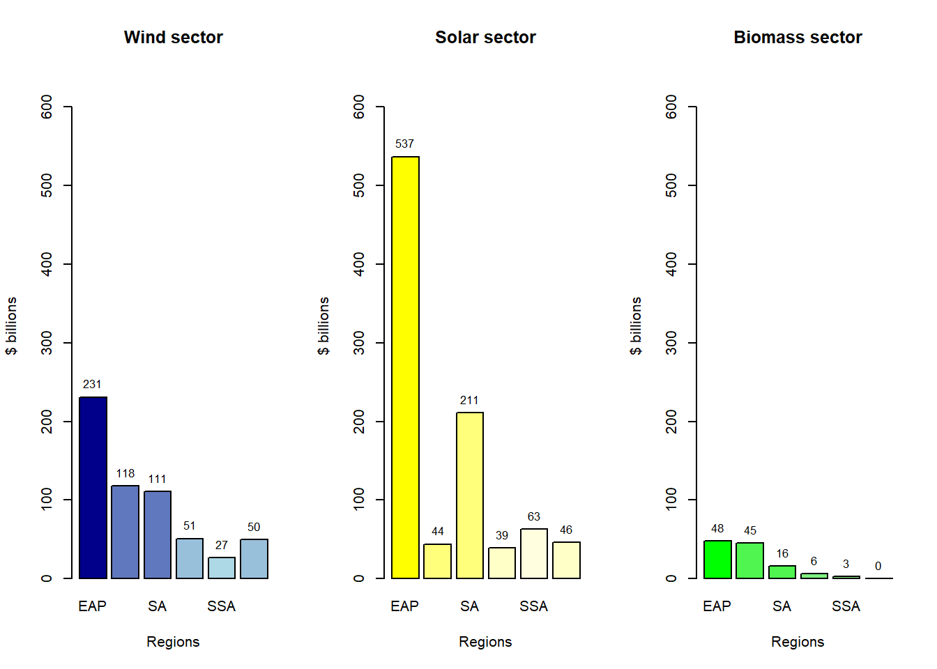
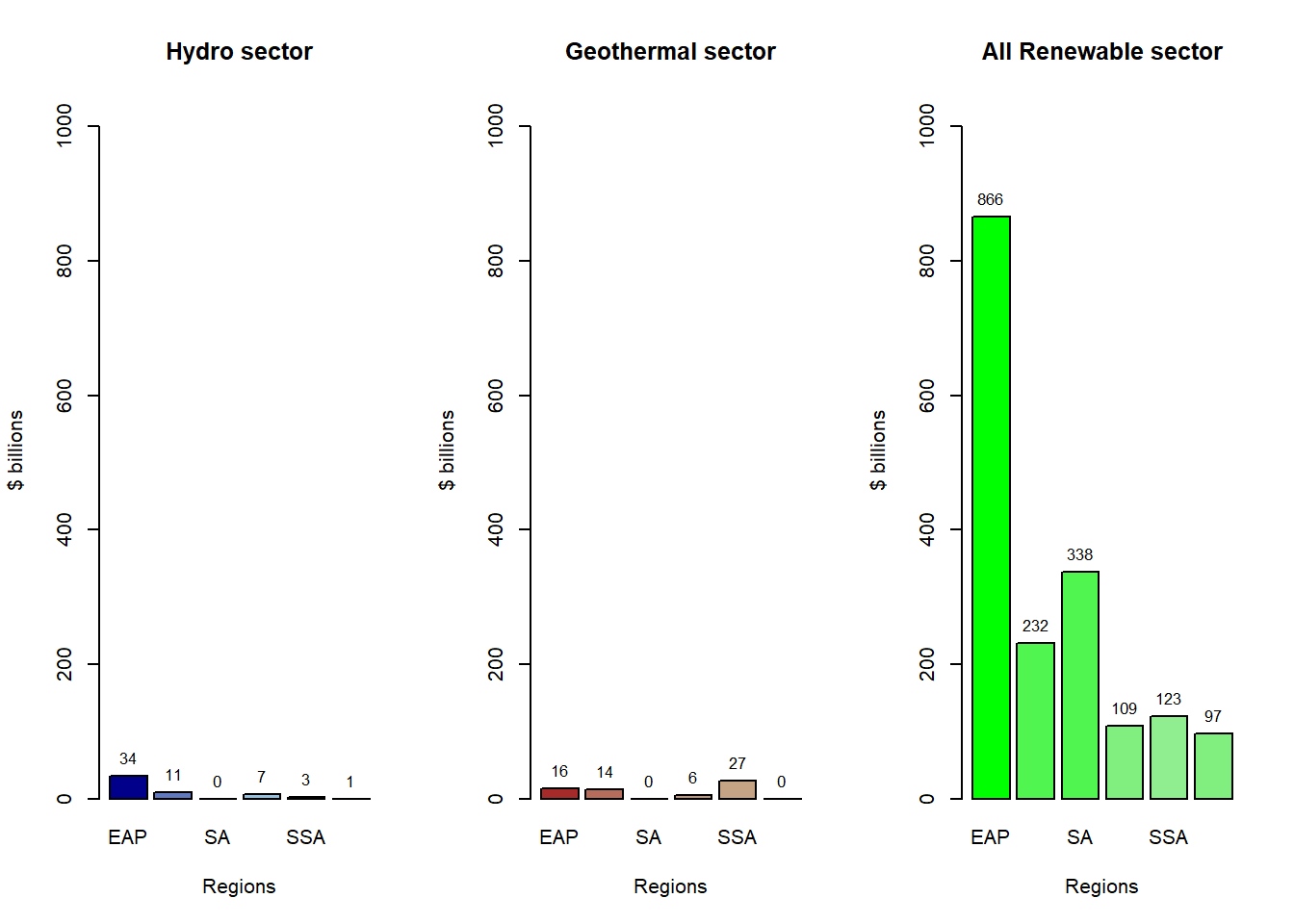
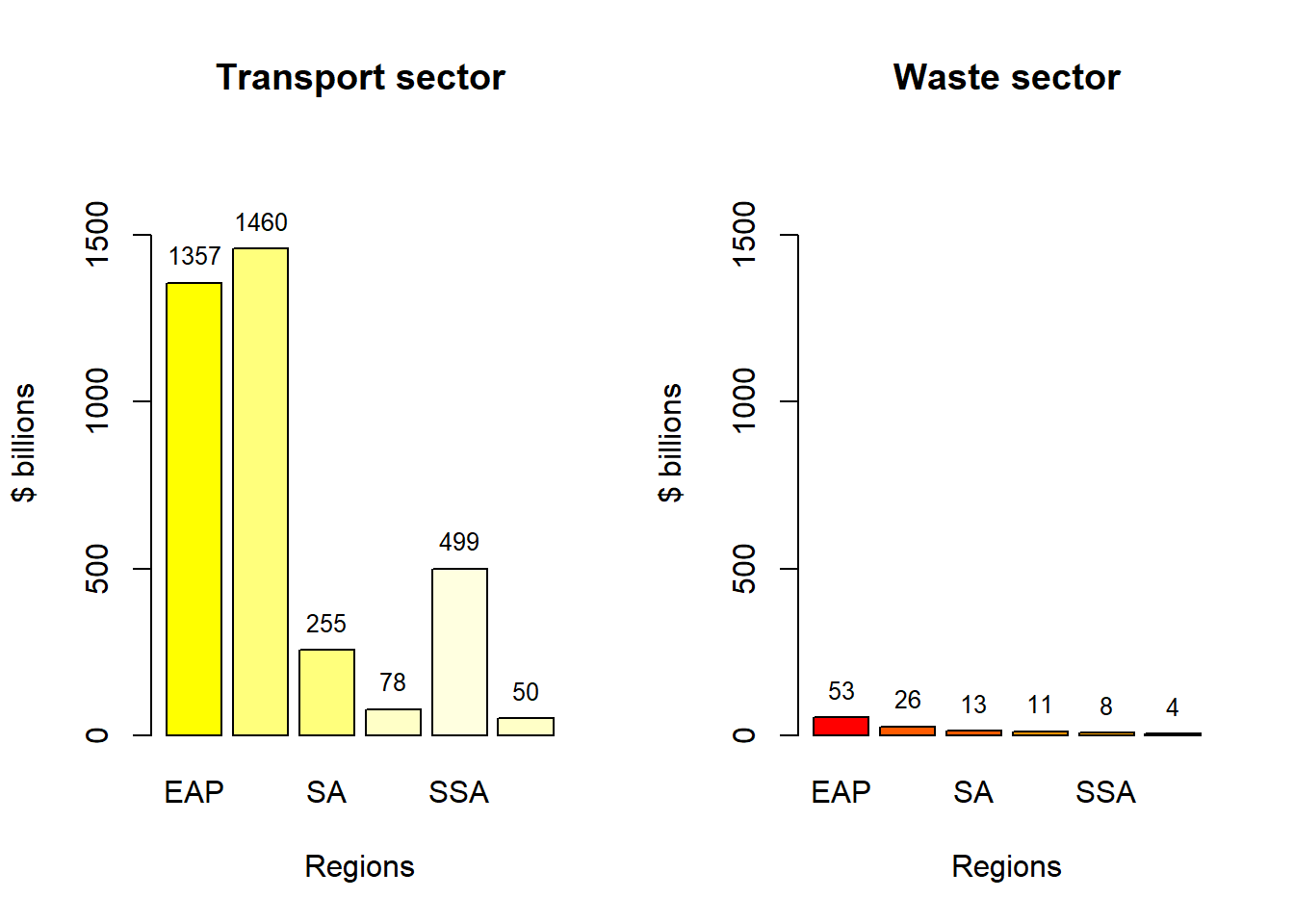
These graphs enable us to analyze which regions require greater investment in specific sectors.
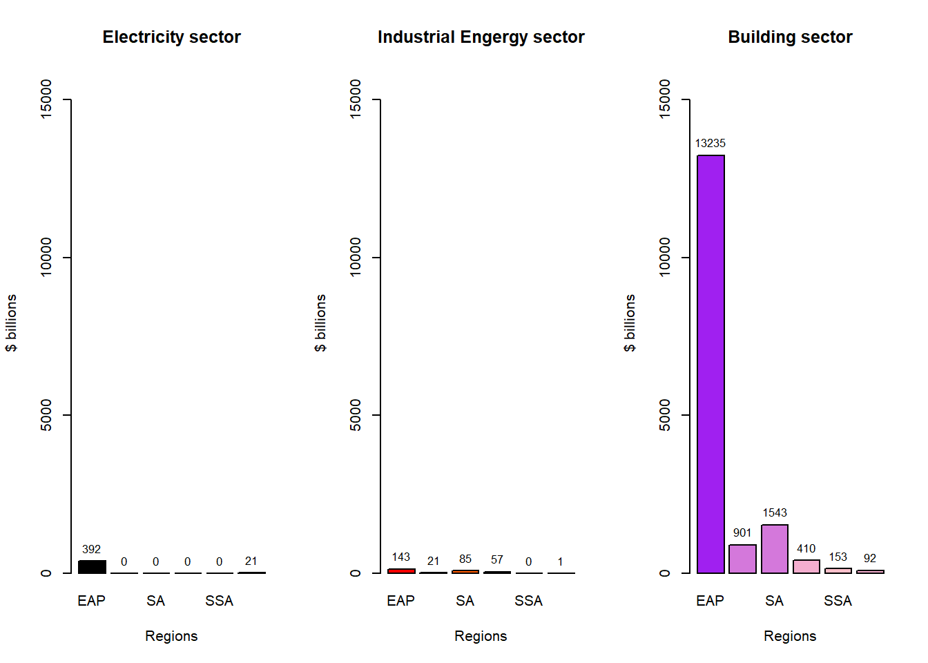
Comparison between different Sectors
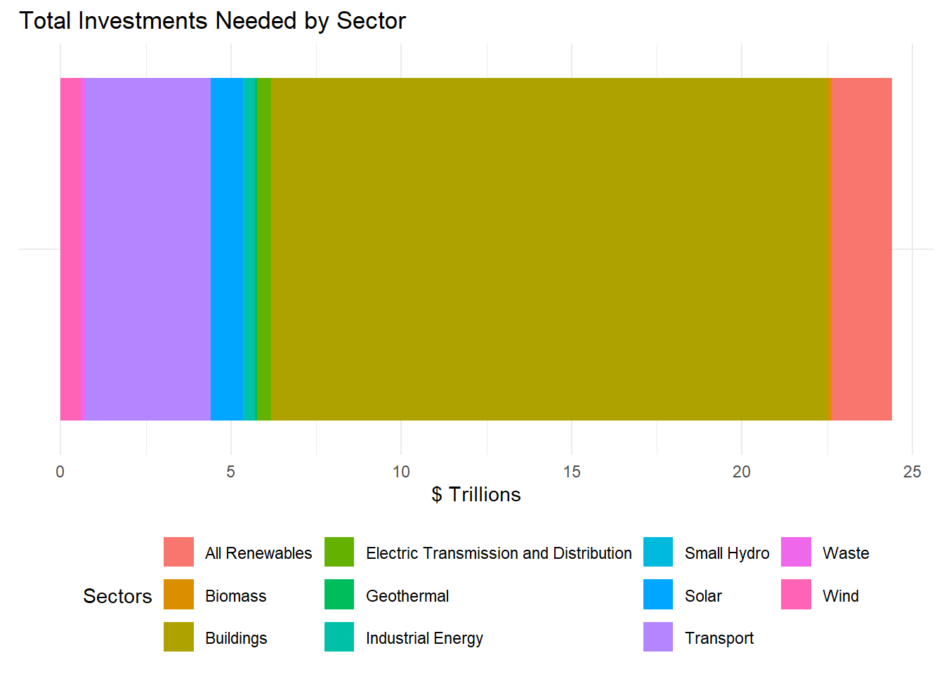
The above graph shows, that the most investment is needed in the Building/Infrastructure sector.
China, Indonesia, the Philippines, and Vietnam have a climate-smart investment potential of $16 trillion, most of which is concentrated in the construction of new green buildings.
Opportunities for new green buildings and energy-efficient retrofits for millions of existing buildings are massive.
Observation:
According to the graphs presented, IFC has projected that approximately $23 trillion will be necessary between the years 2016 and 2030 to achieve the objectives set forth by the Paris Agreement. A significant portion of this investment needs to be allocated to the combined regions of South and East Pacific Asia.
3.2 Climate Tax needed to achieve the targets
As previously discussed, achieving the targets set by the Paris Agreement will require an investment of $23 trillion over the next 15 years.
To generate this substantial amount of funding, one potential strategy the government might consider is imposing a climate tax on the population.
median(DC_WTP)## [1] 192Given the global adult population of 5.16 billion, implementing a climate tax equivalent to the median value of DC_WTP would generate approximately 1 trillion euros annually, which is roughly equal to 1 trillion USD per year.
Over a span of 15 years, this would result in the accumulation of 15 trillion USD, which falls short of the required amount.
Challenge:
- Implementing a climate tax amounting to 192 euros presents a significant challenge in developing and impoverished nations such as India and those in Southeast Asia, regions which collectively account for a substantial portion of the global population.
Given that the survey analyzed in this report was conducted in Europe, if such a tax were to be imposed solely within Europe, the 885 million adult population (including Russia) would contribute approximately $169 billion annually. This would result in a total collection of only $2.5 trillion over a span of 15 years.
Conclusion:
Our study of willingness to pay (WTP) and the financial needs for the Paris Agreement targets highlights challenges and opportunities.
-
The link between WTP and factors like education, gender, and environmental attitudes shows the importance of public awareness. Governments must educate citizens on the urgency of climate action and the benefits of sustainable investments.
-
To address the $23 trillion funding gap by 2030, innovative financing beyond traditional taxes is needed. Governments can boost WTP through policies like tax credits for renewable energy or subsidies for green technologies. Engaging stakeholders across sectors and regions is crucial for global climate resilience and sustainable development.
Achieving these targets requires global collaboration. International partnerships, technology transfers, and capacity-building are key to helping developing countries transition to low-carbon economies. By creating a supportive policy environment and ensuring inclusivity, we can secure a sustainable future.
In conclusion, financial challenges can be overcome with political will and collective action. By raising public awareness, using innovative financing, and fostering international cooperation, we can move towards a climate-resilient world that meets the Paris Agreement goals.
References
-
Population Data(world): https://data.worldbank.org/indicator/SP.POP.1564.TO
-
Population (Europe): https://www.worldometers.info/world-population/europe-population
-
Climate Investment Opportunities in Emerging Markets: An IFC Analysis
Page VI
-
Paris Agreement: https://www.un.org/en/climatechange/paris-agreement